Think of this week’s tip as not one single dish, but rather a series of related snacks; a groaning table of cold hors d’oeuvres or sizzling spicy tapas, with one common theme – they’re all about Excel.

May the F4 be with you

One of the neatest features in Office yet largely hidden; the F4 key repeats the last command without needing to faff about selecting the option from the menu. So what, you might say? Well, what if you’re formatting cells and want to repeat the same format over and over again – you could change one, then use the Format Painter option to apply that to select other cells, or possibly just apply the format you want, then select each additional cell in turn and press F4.

One slight downside is that it only repeats the very last action, so changing a number format and then making it bold wouldn’t be easily repeatable since those are two actions. Still, there are so many uses for this “Magic Key no one knows about”.

CTRL+y does the same thing in case you’ve got one of those annoying keyboards where the function keys do other things, you never know without looking if you’ll be pressing F4 or changing the system volume.

Layouts and Tabs

Now, Windows has lots of tricks for arranging application windows side by side, especially if you have multiple monitors; there’s a particularly shiny new way of doing it in Windows 11 with Snap Layouts. In the context of Excel, that’s OK if you’re using two spreadsheets side by side and you might want to reference or copy data between them, but Excel has its own window-handling functions that could be more useful.

The key scenario here is that you can open the same document in more than one window (by clicking New Window, on the View tab) and then show different parts of it side/side – separate tabs, perhaps, or different areas on the same sheet.

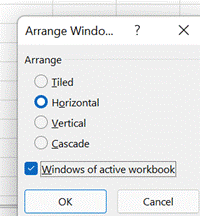
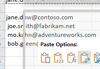
The Synchronous scrolling feature means you can also keep the cursor at the same point in both sheets, making it easier to compare. If you have functions on one tab that depends on data from another, you could change the data in one window and see its impact in real time in the other.

Click on the Arrange All menu option to automatically distribute the open Excel windows, optionally confining the process to just the windows from the active workbook.

Transpose data with paste

It’s a fairly common exercise to take a load of data that’s in one format and want to represent it differently; there is a useful Transpose feature that takes data from columns and paste it back as a row, or vice versa. One useful scenario could be when you want to take the names of everyone who got an email or meeting request and put them in a tabular format.

Start by copying and pasting the names/addresses from Outlook’s To: field into a new cell: you’ll see that is’ one long string of text that needs to be broken down, but in this case, each address is delimited with a semicolon (“;”).

Having selected the cell, go to the Data tab in Excel and choose Text to Columns then choose Delimited and select the semicolon. Once the wizard is complete, you’ll end up with each address in its own column. Now select the multiple cells and copy to clipboard.

Next, put the cursor on a lower row or maybe a new sheet altogether; right-click on the destination cell and under Paste Options, look for the Transpose icon (with the two arrows); hovering over the different icons in this menu will preview what you’re going to do. Click on the icon to commit.

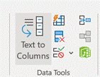
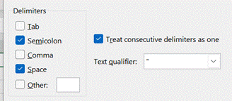
Now you have a list of addresses on their own row, and without the “;”s, but they do have a leading space ahead of all but the first one. It might be quick to correct each line in turn, and there’s always the TRIM function which could be used to tidy stuff up through formulae.

Alternatively, go back to the start of the process, select both Semicolon and space, and choose to combine the two, so the text in the columns is neater.

When you’re happy, remove the original line that had the text in columns, leaving just the separate email addresses on their own rows.

Now, snacks just make you hungry, don’t they?